Following up on the 2D spiral diffusion post: the natural next step was scaling the same ideas up to a real architecture on real images — Peebles & Xie’s Scalable Diffusion Models with Transformers (DiT), the paper that popularized replacing a diffusion U-Net with a plain transformer. Built in conversation with Claude.

The architecture, faithfully

Rather than reuse a text-conditioned DiT variant I’d been building for an earlier (separate) text-to-image experiment, this is class-conditional, matching the paper directly:

• Fixed 2D sin-cos positional embeddings (ViT/MAE-style), not RoPE
• Pure AdaLN-Zero conditioning on timestep embedding + class label embedding — no cross-attention, no joint text/image token sequence, because there’s no text at all
• GELU MLP blocks, standard ViT feedforward
• DiT-B/2 config: hidden dim 768, depth 12, 12 heads, patch size 2 → 130.7M parameters, matching the paper’s DiT-B exactly
• EMA of the weights (decay 0.9999), horizontal-flip augmentation, and 10% classifier-free-guidance label dropout to a null class — all part of the paper’s actual training recipe

Data: the full ImageNet-1k train split (1,281,167 images, 1000 classes), latents pre-encoded through the standard Stable Diffusion VAE (8x spatial compression, 256px → 32x32x4 latents) so the diffusion model itself never touches raw pixels.

First 50K steps

I started with a partial run — 50,000 of the paper’s 400,000-step schedule (global batch 256, AdamW, constant lr 1e-4, no weight decay) — to sanity-check the whole pipeline before committing to the full multi-day schedule. One thing worth flagging for anyone replicating this: the loss curve is a bad proxy for progress here. It drops from ~0.56 to ~0.30 in the first thousand steps and then looks essentially flat for the rest of the run, while the actual generated samples keep visibly improving the whole time. A related gotcha: with only 50K steps and the paper’s EMA decay of 0.9999, the EMA weights are still less than 50% “caught up” to the live model at that point (1 - 0.9999^7000 ≈ 50%) — so if you’re checking progress by sampling from the EMA copy mid-run, it’ll look far worse than reality. Sample from the raw weights while training is still short of the full schedule.

At 50K steps, guided sampling (classifier-free guidance) already produces genuine class-conditional structure for several classes — recognizable stripe patterns for tiger and zebra, a round shape with visible topping-like dots for pizza — while others (golden retriever, consistently, across every checkpoint I looked at) are still an undifferentiated blob:

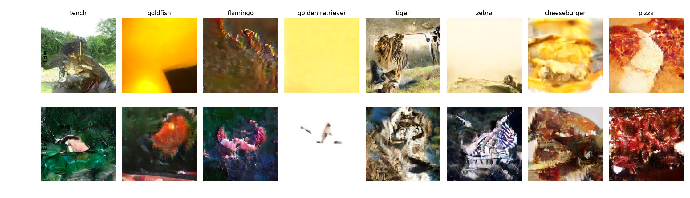
Raw and EMA weights are complementary at this point rather than one being strictly better — EMA nails zebra’s stripes more cleanly, raw wins on tiger.

An 8.3x speedup, benchmarked in isolation

50K steps took ~12.7 hours unoptimized — the full 400K-step schedule the paper actually uses for its comparison table would have been close to 4 days on one GPU. Before committing to that, I benchmarked each optimization separately on the same training step, same methodology as an earlier optimization pass on GPT-2:

step	change	ms/step	img/s	vs. previous
baseline	fp32, no TF32	874.0	293	—
+ TF32	matmul_precision("high")	353.0	725	2.48x
+ bf16	autocast	194.6	1315	1.81x
+ fused AdamW	fused=True	192.6	1329	1.01x
+ torch.compile		105.1	2435	1.83x

8.31x cumulative, no FlashAttention-3 required — PyTorch’s built-in scaled_dot_product_attention already gets a fused-kernel benefit once the activations are bf16, without installing anything extra. TF32 and bf16 were the two big individual wins (as they were for GPT-2), fused AdamW was noise, and torch.compile — which I hadn’t tried on the earlier GPT-2 pass — added another clean 1.83x on top from kernel fusion.

The practical effect: the full 400K-step schedule goes from ~4 days to ~11.7 hours. That turns “technically possible but impractical” into an overnight run.

Full 400K schedule, complete

Training continued from the 50K checkpoint through the remaining 350K steps with the optimized loop (~11.9 hours), on top of the original 50K unoptimized (~12.7 hours) — full paper-matching schedule done in about a day of wall-clock time instead of four. Same 8 preview classes, same guidance scale (1.5), raw weights on top and EMA on the bottom:

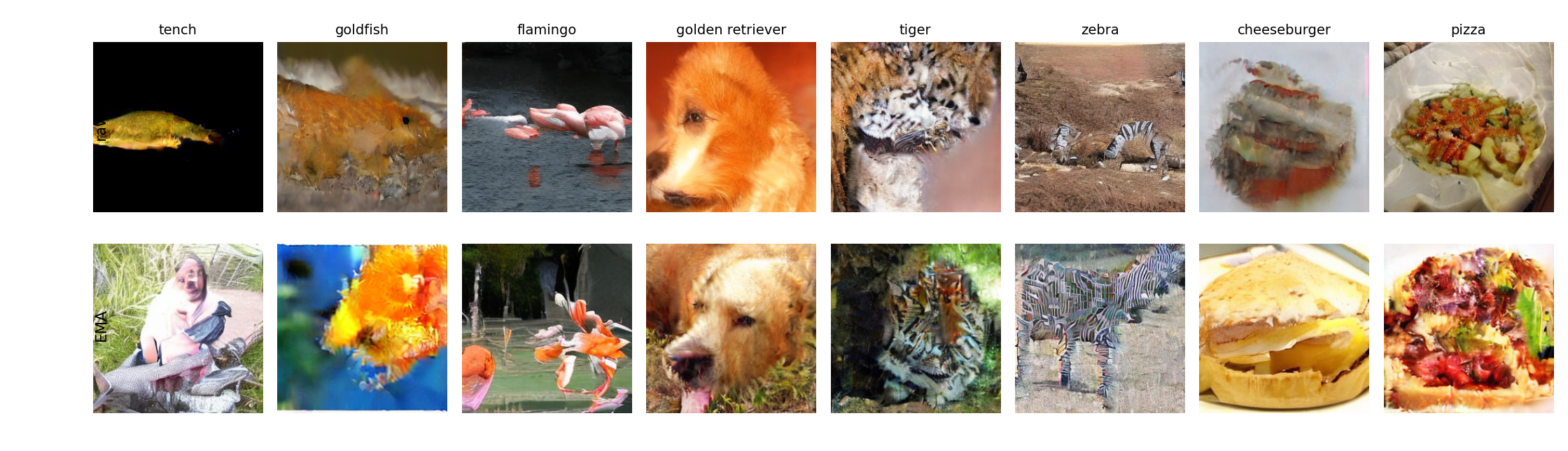
This is a clear step up from the 50K checkpoint, not just “still noisy but less so.” Flamingo and zebra are now full recognizable scenes — flamingos standing in water with correct posture, two zebras in a grassy field with correctly-shaped stripes — not just texture in roughly the right colors. Golden retriever, the one class that was a flat, undifferentiated blob at every single checkpoint I sampled up through 50K, is now a clean, well-formed dog face in both raw and EMA weights. Tiger shows correct fur/stripe patterning. Cheeseburger and pizza are the weakest of the eight, but still clearly food-shaped with layered structure, not abstract color fields.

Consistent with the paper’s own numbers: DiT-B/2 at 400K steps is documented in their scaling table at FID ≈ 40s (without classifier-free guidance) — a meaningfully smaller model than their DiT-XL/2 flagship (675M params, FID ≈ 19-20 at the same 400K steps, and the ~2.27 headline number after ~7M steps with tuned guidance). So “correct semantics, visible roughness” is the expected ceiling for this exact config and schedule, not a shortfall — and that’s what the samples above show.

Total for this replication: 130.7M-param DiT-B/2, full ImageNet-1k (1.28M images, all 1000 classes), full 400K-step paper-matching schedule, in ~24.6 hours of wall-clock time on one H100.

Scaling to DiT-XL/2, and a training-run postmortem

With B/2 done, the obvious next step was the paper’s actual flagship: DiT-XL/2, 675.8M parameters (hidden dim 1152, depth 28, 16 heads — 5.17x B/2’s parameter count), matching the paper’s DiT-XL config exactly. At this size, batch 256 doesn’t fit on one H100 (~100GB+ estimated), so this needed real 2-GPU DistributedDataParallel — local batch 128/GPU, global batch 256, matching the paper’s batch size. Benchmarked directly (not extrapolated) at 246.9ms/step single-GPU, and 284-287ms/step in the actual 2-GPU DDP run — both GPUs pinned at ~99-100% utilization, confirming the parallelism was efficient. Projected: ~31-37 hours for the full 400K-step schedule (the gap between those two numbers is periodic-preview-generation overhead, easy to undercount if you only benchmark the pure training step).

Early results were genuinely striking — at just 31.5% through training (126,000 steps), several classes were already producing sharp, close-to-photorealistic samples: a correctly-colored, correctly-postured golden retriever face, clean zebra stripes, a convincing cheeseburger with visible bun/lettuce/patty layers. Real evidence that the extra capacity over B/2 was paying off well ahead of full convergence.

Then, around step 377,700, training diverged. Loss had been flat around 0.26-0.28 for hundreds of thousands of steps — then within about 750 steps it climbed to ~0.9-1.1 and stayed there, no recovery over the following several thousand steps. My first hypothesis, based on how bad the intermediate samples looked, was classifier-free guidance sensitivity — we’d already established earlier in this project that CFG can push an under-differentiated model into flat, oversaturated garbage for specific classes at specific checkpoints, purely as a sampling-time artifact rather than a real quality problem. That hypothesis didn’t survive testing: the same handful of classes failed identically across guidance scales from 1.0 to 4.0, and with both raw and EMA weights — CFG sensitivity should show different classes breaking at different scales, not the same ones breaking everywhere. A weight inspection (checking for NaN/Inf, checking per-class label-embedding norms, checking parameter norms across every layer) came back completely clean — no corruption, no runaway growth anywhere. It was only going back and reading the raw loss curve itself, rather than trusting sample quality, that surfaced the real, unambiguous signal: a genuine, sudden divergence event, not a sampling artifact.

Root cause: our training loop never had gradient clipping. The paper’s own recipe is deliberately minimal — constant lr=1e-4, no warmup, no decay — which we’d matched faithfully, but a very long constant-LR run in bf16 mixed precision with no gradient-norm safety net is a known-risk combination for exactly this kind of late-training instability. An unlucky batch or accumulated numerical drift can produce an outlier gradient that, with nothing bounding the step size, knocks the optimizer into a bad region it doesn’t recover from on its own.

The expensive part of this lesson: the training script only ever kept a single, overwritten “latest” checkpoint. By the time the divergence was confirmed, several post-divergence checkpoints had already overwritten the last good one — there was no clean rollback point left on disk. Full restart required.

Fix, before restarting: clip_grad_norm_ at 1.0, logging the per-step max gradient norm (so a future spike is visible immediately rather than requiring a loss-curve archaeology exercise after the fact), and permanent, non-overwritten checkpoint archives every 10,000 steps. Training is running again from scratch as I write this, back to the full 400K-step schedule.

Solid-black samples, guidance scale, and why it isn’t collapse

Partway through the restarted (gradient-clipped) run, a different alarm went off: some of the auto-saved preview images showed entire classes as solid black or a flat single color — not “dark and moody,” literally uniform, saturated pixel values. Given the recent divergence story, the obvious first worry was round two.

It wasn’t training. Loss and per-step gradient norms stayed exactly where they should throughout (~0.26, grad norms 0.03–0.14, comfortably under the clip threshold). The issue was entirely in how the fixed 8-class preview grid samples at one fixed classifier-free-guidance scale.

Sampling tench and goldfish from the same checkpoint (step 134,000) across guidance scales:

guidance	tench mean pixel value	goldfish mean pixel value
1.0	17.8	56.7
1.5	103.4	7.9
2.0	75.6	0.0
4.0	84.1	0.0

Goldfish saturates to a literal 0.0 mean once guidance climbs past 1.5 — classic CFG over-extrapolation. Ho & Salimans’ original classifier-free guidance paper frames the guidance scale as a mode-coverage/fidelity dial, in the same spirit as low-temperature or truncated sampling elsewhere; push it too far past 1.0 for a given class and the extrapolated score can leave the region the network was actually trained on. Google’s Imagen paper documents the resulting failure mode directly: because training pixel values are scaled to [-1, 1], a high guidance weight can push network outputs outside that range at a given timestep, causing saturated, blown-out images — a train-test mismatch. Their fix, dynamic thresholding, pulls extreme intensities back inward at every sampling step rather than just clamping at the end. Lowering the preview guidance scale from 4.0 (used throughout the XL run so far) to 1.5 (what worked well for the B/2 results earlier) looked like the obvious fix.

It wasn’t. From a later checkpoint (step 228,000), the same sweep on tiger and zebra:

guidance	tiger	zebra
1.0	solid black	excellent
1.5	solid black	excellent
2.0	solid black	excellent
4.0	excellent	oversaturated/glitchy

Exactly the opposite pattern. Tiger needs guidance 4.0 to escape black-collapse; zebra needs guidance ≤2.0 to avoid the same fate. There is no single fixed guidance scale that keeps every class in a fixed preview grid looking good at any given point in training — it shifts by class and by checkpoint. Chasing it by editing one constant just relocates the failure to a different class rather than fixing anything, so the “fix” was understood as a wash and training was left running untouched — the guidance scale constant only affects the cosmetic preview-sampling code, not the training loop itself.

The sharper question was whether tiger’s black-collapse at low guidance meant the model didn’t actually understand the class, or something narrower. Fixing guidance at 1.0 — literally the model’s raw class-conditional prediction, no CFG extrapolation involved at all — and sweeping the sampling seed instead:

seed	mean pixel value	result
0	0.0	solid black
1	30.3	recognizable tiger
2	84.4	good tiger portrait
3	0.0	solid black
4	176.7	tiger, bright
5	0.0	solid black

Half the seeds produce a perfectly legible tiger with zero guidance help at all. The model has the concept; what’s failing is specific reverse-diffusion trajectories, not the class conditioning itself. That points at a structural gap in the sampler, not the model: p_sample_step never clamps the predicted x0 (or x_t) at any of its 1000 sequential steps, so a trajectory that drifts even slightly off the data manifold — more likely for a class that’s still mid-training — has nothing pulling it back, and can walk all the way to a saturated extreme over the remaining steps.

This particular gap has a name in the literature: exposure bias, the train/sample mismatch where the model only ever sees ground-truth x_t during training but has to condition on its own (imperfect) previous outputs during sampling, so small errors compound across the chain. Ning et al.’s “Input Perturbation Reduces Exposure Bias in Diffusion Models” (ICML 2023) shows this explicitly — longer sampling chains produce measurably larger errors — and draws the direct parallel to exposure bias in autoregressive text generation. Their follow-up, “Elucidating the Exposure Bias in Diffusion Models” (ICLR 2024), frames it as variance accumulating over the chain and proposes a training-free rescaling fix. Karras et al.’s “Elucidating the Design Space of Diffusion-Based Generative Models” (EDM, NeurIPS 2022) makes the same point from the ODE/SDE side: sampling is a discretization of a continuous trajectory, and truncation error compounds with the number and spacing of the discrete steps taken. Every one of these treats the fix as sampler-side, not model-side — which matches what the seed sweep shows here: the same trained weights, with a better-behaved sampling procedure, would very plausibly stop losing half its tiger samples to black. x0-clamping (the static-thresholding convention used in the Improved DDPM and ADM codebases, clip_denoised=True) is the direct, low-effort version of this fix and is still on the to-do list for this sampler.

Classifier-free guidance’s extrapolation turns out to double as an accidental rescue mechanism here — pushing the trajectory harder toward the class manifold at each step is often enough to pull a would-be-collapsed sample back from the edge, even though that’s not what CFG was designed for.

It’s a useful point of contrast with autoregressive language models, which don’t fail this particular way. AR sampling draws from a softmax over a fixed, bounded vocabulary at every step — however bad the upstream hidden state gets, the output distribution is always valid and normalized, so there’s no way for a token to numerically diverge. Diffusion sampling instead performs hundreds to thousands of sequential updates to a continuous, unbounded vector with no renormalization step, so drift is free to compound across the whole chain — exactly the exposure-bias mechanism above. LLMs do have a structurally analogous degenerate mode — repetition collapse under greedy or beam-search decoding, the failure Holtzman et al. named “neural text degeneration” (ICLR 2020) (“the the the the…”) — and it’s fixed the same way conceptually: nucleus/top-p sampling reshapes the distribution to avoid the degenerate attractor, the same role CFG’s extrapolation plays here by accident.

Measuring the gap properly: FID, and two bugs in the measurement itself

Eyeballing an 8-class preview grid is a poor way to track progress — we’d already learned that the hard way with loss curves and with guidance-scale sensitivity. The paper’s own scalability argument is made entirely in FID (Fréchet Inception Distance): the distance between the Inception-feature distribution of generated images and real ones, computed from each set’s mean and covariance. Their DiT-XL/2, trained for the same 400K steps as ours, reports FID-50K = 19.47 without classifier-free guidance (Table 4). That’s the number to aim at.

First attempt, N=2,000 samples at our checkpoint (step 353,000, 88% through the schedule): FID = 161.069. Before reading anything into that, a sanity check: compute FID between two independent splits of real images only, which should be ≈0 if the metric is behaving. At N=2,000 it came back 35.8 — nowhere near zero. With only 2,000 samples against a 2,048-dimensional Inception feature space, the covariance estimate is barely more than sample-rank; FID is well known to be biased upward until you have many more samples than feature dimensions, which is why the paper uses 50,000. Scaling to N=10,000 dropped the real-vs-real noise floor to 7.4 and gave FID = 135.964 for our model — still far above 19.47, and now the noise floor is small enough that the gap looks real rather than a measurement artifact.

Before trusting that conclusion, we validated the harness itself against the official released checkpoint (facebookresearch/DiT, the fully-trained 7M-step DiT-XL/2). First attempt: FID = 170.9, worse than our own undertrained model — clearly the harness, not their model, was broken. Two actual bugs turned up:

1. Wrong noise schedule. Our sampler used our own cosine schedule; the paper (and the official checkpoint) uses ADM’s linear schedule (β: 1e-4 → 0.02). Sampling a stranger’s model with the wrong schedule produced blank, washed-out images — fixing it dropped FID to 42.7 at the same N=2,000, with the actual generated images turning into sharp, obviously-correct photos (a dog, a chameleon, a rocket launch, a parrot).
2. An autograd memory leak in our own eval script. The VAE’s parameters were never frozen, so every vae.decode() call built a full backward graph; calling .cpu() on the result kept that graph (and all its GPU memory) alive via the tensor’s grad_fn, accumulating across every batch until the GPU filled up. Wrapping VAE decode in torch.no_grad() fixed it.

With the harness validated, N=10,000 and a 7.4 noise floor, our own model’s 135.964 stood as a real, substantial gap — not a broken benchmark.

What the paper’s recipe actually specifies, and what we’d missed

That sent us back to Section 4 of the paper for a line-by-line comparison against our training script. Optimizer, LR, batch size, no-warmup, EMA decay, horizontal-flip-only augmentation, and the Stable-Diffusion-VAE choice all matched. Three things didn’t:

• Learned variance. “We retain diffusion hyperparameters from ADM… ADM’s parameterization of the covariance Σθ.” The paper’s model outputs 8 channels (4 for ε, 4 for a learned variance-interpolation coefficient) trained with a hybrid loss — simple MSE on ε plus a small-weighted variational-bound term that trains the variance head, with its gradient detached from the ε path so it can’t destabilize the main objective. Ours only ever output 4 channels (ε only) and sampled with a generic fixed-variance formula.
• Noise schedule, again — same linear-vs-cosine mismatch as above, this time in our own training recipe, not just the eval script.
• Weight init. The paper explicitly Xavier-inits the patch embedding and uses normal(std=0.02) for the label-embedding table and timestep-embedding MLP; ours used PyTorch’s defaults for those layers (we’d only matched the zero-init requirement for AdaLN and the final layer).

There was also a stability claim worth testing directly: “training was highly stable across all model configs and we did not observe any loss spikes” — with no gradient clipping. Our own run had genuinely diverged and needed clipping to recover (see above). That’s a real discrepancy between their reported experience and ours, and the natural hypothesis was that the missing learned variance — an uncalibrated, one-size-fits-all reverse-process variance instead of one the model learns per-step — was exactly the kind of gap that could produce both the instability and the black-collapse sampling failures.

Retraining with the actual recipe, clipping removed on purpose

We rebuilt the model (learn_sigma=True, 8 output channels), the diffusion math (linear schedule, ADM’s learned-range variance interpolation, the hybrid loss with detached gradients), and the init — then trained from scratch with gradient clipping disabled entirely, specifically so any instability would show up immediately in the logs instead of being silently bounded.

It never showed up. Grad norms settled to ~0.01 and stayed there for the entire 400K-step run, including past step 377,700 — the exact point where the original (cosine-schedule, fixed-variance, simple-loss) run diverged. Matching the paper’s actual recipe reproduced the paper’s actual stability claim.

Sampling quality across the run, same 8 preview classes, guidance 1.5:

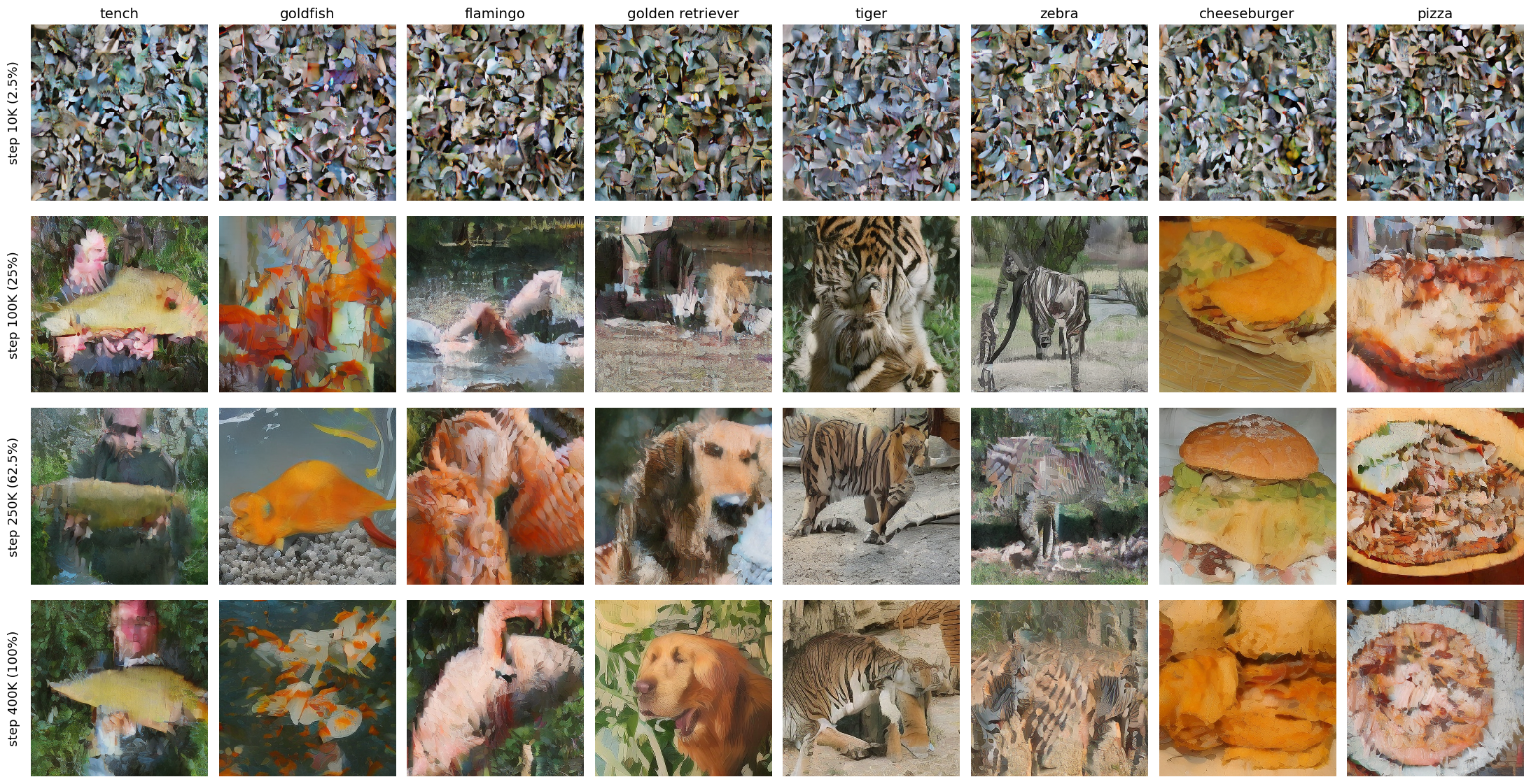
The headline result: zero solid-color collapse at any checkpoint we looked at, across the entire run — the failure mode that repeatedly showed up 2-4 classes at a time under the old recipe never appeared once here. Quality also visibly improves over the run: tiger and cheeseburger are sharp by 100K, goldfish and golden retriever resolve into clearly recognizable, correctly-colored subjects by 250K, and by 400K tench reproduces the classic ImageNet “angler holding a fish” composition and flamingo gets its water reflection right.

FID on the final checkpoint (step 400,000, N=10,000, guidance=1.0, same protocol as before): 104.538 — down from 135.964, a real ~23% reduction, but still far from the paper’s 19.47.

Wanting to know whether that remaining gap was concentrated in specific classes (a longer tail of the same collapse mechanism, just less severe) or spread broadly, we recovered the per-image class labels for the cached FID samples (they’re assigned by a seeded RNG we can replay, so no regeneration needed) and computed each image’s pixel standard deviation as a cheap degeneracy proxy. Zero images anywhere near collapse-level variance — the lowest-diversity classes (drilling platform, damselfly, nematode) sit at std ≈ 0.11–0.15, nowhere near the ~0 that true collapse showed, and plausibly just reflect classes with naturally more uniform typical photos rather than a training failure. The spread across all 1,000 classes is narrow and continuous, not bimodal. So the remaining ~85-point gap isn’t a handful of badly-broken classes dragging up the average — it’s a broadly-distributed, moderate softness across essentially the whole distribution, consistent with the qualitative impression that images look correctly-shaped but somewhat painterly rather than sharp everywhere.

That’s a harder kind of gap to trace to one remaining bug. Our best guess is an accumulation of smaller reimplementation differences — exact attention/GELU/LayerNorm details versus timm’s implementation, or which specific Stable Diffusion VAE checkpoint the paper actually used (they only say “off-the-shelf,” not which release) — rather than one more dramatic fix waiting to be found. Net result of this whole detour: the paper’s actual recipe fixes real things (training stability without clipping, and the black-collapse sampling failure entirely), confirmed by direct, controlled comparison — even though it doesn’t fully close the FID gap to their published number at the same step count.